On this page
Two features and a straight line are enough to build the classifier in my Reto 4 notebook. Finding that line takes us from dot products in feature space to a convex loss in parameter space. This field guide follows that path in 11 sections, pairing the original notebook figures and results with browser-based experiments.
The interactive labs run in your browser with JavaScript and local assets.
The classification problem
00 / ORIGINAL NOTEBOOK
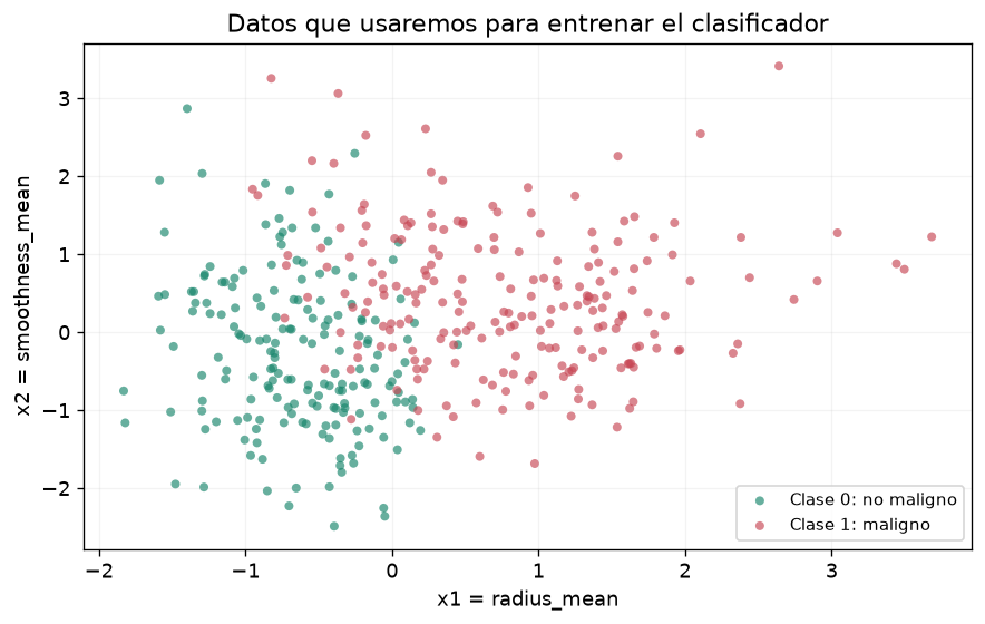
The notebook trains a binary classifier from radius_mean and smoothness_mean to predict pronostic: 1 for malignant, 0 for non-malignant. It optimizes probabilities, then evaluates the resulting linear decision boundary.
392 × 2
Z: 392 × 3
The whole problem is a dot product, repeated 392 times
01 / LINEAR ALGEBRA
Each observation begins as a 2D feature vector . The notebook appends a constant 1, producing a 3D augmented vector . That extra coordinate lets the model learn an intercept without a separate operation.
One observation
The output sᵢ is a scalar called a logit or score. Geometrically, w₁ and w₂ define the orientation of a line; w₃ translates it.
All observations simultaneously
Each row of Z is one observation. Each column is a model input (two features and a constant).
Try a matrix multiplication by handUse the sliders to change one augmented row
This is a synthetic example feature vector evaluated with the actual optimized weights. Its computed probability is illustrative, not a record taken from the original dataset.
Z @ w. More importantly, derivatives become compact: and . Both are built from the same matrix Z.Three coefficients determine one straight line
02 / FEATURE SPACE
Logistic regression is called “regression”, but the notebook uses it for binary classification. First compute ; then turn it into . The class threshold of 0.5 corresponds exactly to s = 0.
Interactive decision boundaryTeaching dataset · not the original 392 records
Why does the notebook minimize cross-entropy?
03 / PROBABILITY & LOSS
We want high probability on the true class, not just the right side of a threshold. With a Bernoulli model, the likelihood of label is . Minimizing negative log-likelihood gives the binary cross-entropy (BCE) used in the notebook.
One prediction, two loss choicesCompare BCE vs squared probability error
Sigmoid: turns a logit into a probability
Loss as a function of the logit s
BCE has the right probabilistic interpretation
Its average is the negative log-likelihood of the training labels, so minimizing BCE is maximum likelihood estimation for Bernoulli observations. It heavily penalizes confident wrong predictions and rewards calibrated probabilities.
Why not optimize accuracy directly?
Accuracy jumps only when a prediction crosses 0.5. As a function of w, it is a discontinuous, piecewise-constant objective with no useful ordinary gradient. BCE is smooth, differentiable and convex in w for this linear-logit model.
Why np.logaddexp? It computes stably even for very large positive s. Algebraically, is exactly the same BCE, expressed in logits. A direct np.log(1+np.exp(s)) may overflow. The notebook stabilizes its loss; for very extreme logits the standalone sigmoid could also be implemented more robustly with scipy.special.expit.
Why is the loss a convex curve, and why is that powerful?
04 / CONVEX ANALYSIS
A convex function lies at or below the straight chord connecting any two points on its graph. For a twice differentiable one-variable function, a nonnegative second derivative everywhere is enough to prove convexity. Logistic cross-entropy satisfies that condition as a function of the logit.
Move the chord: visualize Jensen's inequalityExperiment with BCE and an alternative
From a convex curve to a convex surface
Every logit is affine in w. A convex loss composed with an affine function remains convex. An average of convex functions remains convex. Therefore, f(w) is convex throughout ℝ³.
Why the sigmoid isn't the convex object
The sigmoid is S-shaped: it changes curvature. Its graph is not globally convex. What is convex is cross-entropy applied to the linear score as a function of the parameters. Squared error applied to sigmoid probabilities generally loses this guarantee.
What exactly happens inside minimize?
05 / THE OPTIMIZER
The notebook calls minimize(perdida, w0, args=(Z, t), callback=guardar_perdida). Because there are no bounds, constraints, Jacobian or method specified, SciPy chooses BFGS by default for this unconstrained problem, numerically approximates derivatives and iteratively improves w.
Gradient descent: useful baseline
It follows the local steepest-descent direction. The step-size α affects stability: too small is slow; too large can overshoot.
BFGS: the notebook's method
Bₖ is a changing approximation of the inverse Hessian. BFGS adapts to curvature and uses a line search. It does not require you to supply the true Hessian.
w₀ = (0,0,0)
f(wₖ)
∇f(wₖ)
and line-search step
check stop
Optimizer sandbox: run the iterations yourselfToy logistic dataset · true computed losses, not historical notebook steps
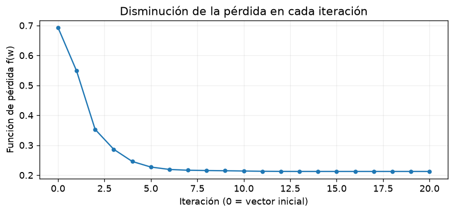
Important: This executes a minimal gradient-descent or inverse-Hessian BFGS demonstration in JavaScript on deterministic toy observations. SciPy's production BFGS has a more sophisticated line search, stopping conditions and derivative approximations. The notebook's actual run is still the separate 20-iteration plot above.
What is saved by the callback?
The notebook initializes historial_f = [perdida(w0,Z,t)] manually and appends a loss each time the callback receives an updated vector. callback is for observation/recording; it does not change the mathematical objective.
Why did it stop?
Its output reports success=True, 20 iterations, , and . A small gradient indicates little first-order improvement remains; combined with convexity, this supports a global minimizer.
The gradient is a direction; the Hessian is a curvature map
06 / DIFFERENTIAL GEOMETRY
The notebook derives the gradient and Hessian analytically for . The gradient is a 3-vector indicating how sensitive the loss is to each coefficient. The Hessian is a symmetric 3×3 matrix describing how the gradient changes as we move in parameter space.
Walk around the convex bowlSecond-order Taylor approximation at the actual notebook optimum
Fix w₃ at its optimized value. Move w₁ and w₂ near w*. Using the actual Hessian matrix, the local loss is approximated by . The colors and ellipses are not exact global loss contours because the original 392 CSV rows are absent from this HTML.
Real Hessian at w*
Off-diagonal terms describe interaction between parameters; symmetry follows from continuous mixed partial derivatives.
Actual Hessian eigenvalues
All positive → positive definite at w*. Eigenvectors identify principal directions; eigenvalues measure curvature along them. A small eigenvalue means a relatively flat direction.
Remember: is small but not exactly zero because this is numerical optimization. The Hessian is not expected to be zero at the minimum; a positive Hessian is the signature of an upward-curving valley.
Why loss and classification metrics answer different questions
07 / EVALUATION
Loss evaluates the quality of predicted probabilities. A confusion matrix evaluates hard decisions after thresholding at 0.5. The notebook reports both on the same training observations, so these are training results—not evidence of generalization to unseen patients.
Explore the original confusion matrixClick any cell to inspect its meaning
Choose a cell
The diagonal contains correct classifications; the off-diagonal cells contain errors.
What the notebook truly demonstrates
BFGS finds a lower training BCE than the prior candidates. The optimized model makes 359 correct hard predictions on the 392 training rows, at the notebook's fixed threshold.
What you would test next
Use held-out test data or cross-validation; examine ROC-AUC, precision–recall trade-offs and calibration, and choose the decision threshold based on the cost of each error. None of those tests were carried out in the Reto 4 notebook.
Which candidate wins, and by what definition?
08 / THE FOUR MODELS
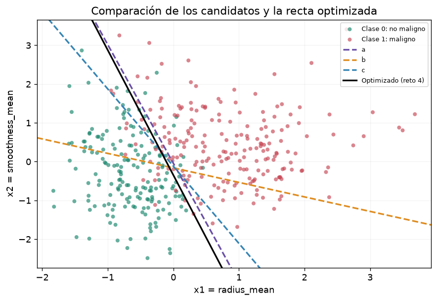
The notebook compares three fixed candidates from Reto 3 with the BFGS solution from Reto 4. They are evaluated on the same Z and t, so their losses are directly comparable.
Original notebook valuesSmaller cross-entropy and gradient norm are preferable here
| Candidate | Weights (w₁,w₂,w₃) | ‖∇f(w)‖ | Smallest λ(H) |
|---|---|---|---|
| Optimized | (5.1718, 1.6045, 0.5622) | 0.000004 | 0.006033 |
| a | (4.0364, 1.3192, 0.0603) | 0.027494 | 0.011861 |
| c | (1.0000, 0.5020, 0.0603) | 0.159099 | 0.134484 |
| b | (1.3450, 3.5970, 0.5880) | 0.245193 | 0.014797 |
The optimized loss is about 4.31% lower than candidate a. Every reported Hessian in this comparison is positive definite at the evaluated point. This does not imply all four have equal fit or gradients.
Can you reason through the whole chain?
09 / CONCEPT CHECKS
Try to answer each question before expanding it. Each answer is tied to a specific idea used by the notebook.
Why does Z have 3 columns if there are only 2 features?
If a point is classified correctly, does its loss have to be small?
The sigmoid curve has an S shape. How can logistic regression be convex?
Why does a positive definite Hessian at the solution matter?
Does SciPy's BFGS use the hessiana(w,Z,t) function in this notebook?
Can 91.58% training accuracy be interpreted as clinical accuracy on future patients?
The notebook, line by line in mathematical terms
10 / CODE MAP
Core functions, matching the notebook implementation
def sigmoide(s):
    return 1 / (1 + np.exp(-s))
def perdida(w, Z, t):
    s = Z @ np.asarray(w, dtype=float)
    return np.mean(np.logaddexp(0.0, s) - t * s)
def gradiente(w, Z, t):
    y = sigmoide(Z @ w)
    return Z.T @ (y - t) / len(t)
def hessiana(w, Z, t):
    y = sigmoide(Z @ w)
    pesos = y * (1 - y)
    return (Z.T * pesos) @ Z / len(t)
w0 = np.zeros(3)
historial_f = [perdida(w0, Z, t)]
def guardar_perdida(w):
    historial_f.append(perdida(w, Z, t))
resultado = minimize(perdida, w0, args=(Z, t),
                     callback=guardar_perdida)
w_opt = resultado.x
What each object means
resultado.x is the parameter vector; resultado.fun is the objective value at that vector; resultado.nit counts optimizer iterations; resultado.success is its success flag. The callback records iterates, but function evaluations can be more numerous than iterations.
Optional clarity improvement
resultado = minimize(
    perdida, w0,
    args=(Z, t),
    method="BFGS",
    jac=gradiente,
    callback=guardar_perdida
)
This is an additional suggestion, not the original code. Passing jac=gradiente provides the analytical gradient, avoiding BFGS's need to estimate it by finite differences. It can change numerical details of the run.
Source: Reto 4 (Reto4LuisOtalora.html). The training figures and results come from the notebook. The interactive labs identify their teaching data and local quadratic approximation. The clinical labels are part of an educational dataset.